Bounded Biharmonic Weigths for Real-Time Deformation
本文共 22297 字,大约阅读时间需要 74 分钟。
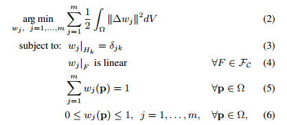
3.1 Formulation
![refered from [1] at page 5](https://img-blog.csdn.net/20160603032113600)
3.4 Implementation
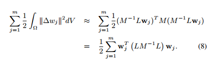
![refered from [1] at page 17](https://img-blog.csdn.net/20160603032900609) [refered from [1] at page 17] Here, we let uj=Δωj .
[refered from [1] at page 17] Here, we let uj=Δωj . ![refered from [2] at formula (9)](https://img-blog.csdn.net/20160603033751059)
∑j=1m12∫Ω∥Δωj∥2dV=∑j=1m12∫Ω∥vj∥2dV
According to formula (2.60), it equals to: ∑j=1m12∫Ω∥vj∥2dV=12∑j=1m∫Ω∥vj∥2dV=12∑j=1mvTjMvj
According to the left-bottom equation of (9), we can easily get vj : vj=M−1Luj=M−1Lwj
} Then, I would like to analysis the matlab source code:
% This is a script that demos computing Bounded Biharmonic Weights% automatically for a 2D shape.%% This file and any included files (unless otherwise noted) are copyright Alec% Jacobson. Email jacobson@inf.ethz.ch if you have questions%% Copyright 2011, Alec Jacobson (jacobson@inf.ethz.ch)%% NOTE: Please contact Alec Jacobson, jacobson@inf.ethz.ch before% using this code outside of an informal setting, i.e. for comparisons.%%%%%%%%%%%%%%%%%%%%%%%%%%%%%%%%%%%%%%%%%%%%%%%%%%%%%%%%%%%%%%%%%%%%%%%%%%%%%%%% Load a mesh%%%%%%%%%%%%%%%%%%%%%%%%%%%%%%%%%%%%%%%%%%%%%%%%%%%%%%%%%%%%%%%%%%%%%%%%%%%%%%%% input mesh source: *.obj, *.off, *.poly, or *.pngmesh_source = 'woody.obj';% should input mesh be upsampledupsample_mesh = false;if(~isempty(regexp(mesh_source,'\.(off|obj)$'))) % load a mesh from an OBJ [V,F] = load_mesh(mesh_source); %顶点存储V中,在2维空间中,V为 #V * 2矩阵 %面的索引存储在F中,在2维空间中,F为 #F * 3矩阵 % only keep x and y coordinates, since we're working only in 2D V = V(:,1:2);elseif ~isempty(regexp(mesh_source,'\.poly$')) % load a mesh from a .POLY polygon file format % Triangulate in two-passes. First pass with just angle constraint forces % triangles near the boundary to be small, but internal triangles will be very % graded [V,F] = triangle(mesh_source,'Quality',30); % phony z-coordinate V = [V, zeros(size(V,1),1)]; % compute minimum angle min_area = min(doublearea(V,F))/2; % Use minimum area of first pass as maximum area constraint of second pass for % a more uniform triangulation. probably there exists a good heuristic for a % maximum area based on the input edge lengths, but for now this is easy % enough [V,F] = triangle(mesh_source,'Quality',30,'MaxArea',min_area);elseif ~isempty(regexp(mesh_source,'\.png$')) % load a mesh from a PNG image with transparency [V,F] = png2mesh(mesh_source,1,50);end% upsample each triangleif(upsample_mesh) [V,F] = upsample(V,F);end%%%%%%%%%%%%%%%%%%%%%%%%%%%%%%%%%%%%%%%%%%%%%%%%%%%%%%%%%%%%%%%%%%%%%%%%%%%%%%%% Place controls on mesh%%%%%%%%%%%%%%%%%%%%%%%%%%%%%%%%%%%%%%%%%%%%%%%%%%%%%%%%%%%%%%%%%%%%%%%%%%%%%%%% display meshtsurf(F,V)axis equal;fprintf( ... ['\nCLICK on mesh at each location where you would like to add a ' ... 'point handle.\n' ... 'Press ENTER when finished.\n\n']);% User clicks many times on mesh at locations of control pointstry [Cx,Cy] = getpts;catch e % quit early, stop script returnend% store control points in single #P by 2 list of pointsC = [Cx,Cy];%%%%%%%%%%%%%%%%%%%%%%%%%%%%%%%%%%%%%%%%%%%%%%%%%%%%%%%%%%%%%%%%%%%%%%%%%%%%%%%% Bind controls to mesh%%%%%%%%%%%%%%%%%%%%%%%%%%%%%%%%%%%%%%%%%%%%%%%%%%%%%%%%%%%%%%%%%%%%%%%%%%%%%%%% Note: This computes the "normalized" or "optimized" version of BBW, *not* the% full solution which solve for all weights simultaneously and enforce% partition of unity as a proper contstraint. % Compute boundary conditions[b,bc] = boundary_conditions(V,F,C);% Compute weightsif(exist('mosekopt','file')) % if mosek is installed this is the fastest option W = biharmonic_bounded(V,F,b,bc,'conic');else % else this uses the default matlab quadratic programming solver W = biharmonic_bounded(V,F,b,bc,'quad',true);end% Normalize weightsW = W./repmat(sum(W,2),1,size(W,2));%%%%%%%%%%%%%%%%%%%%%%%%%%%%%%%%%%%%%%%%%%%%%%%%%%%%%%%%%%%%%%%%%%%%%%%%%%%%%%%% Deform mesh via controls%%%%%%%%%%%%%%%%%%%%%%%%%%%%%%%%%%%%%%%%%%%%%%%%%%%%%%%%%%%%%%%%%%%%%%%%%%%%%%%% Display mesh and control points and allow user to interactively deform mesh% and view weight visualizations% Commented out are examples of how to call "simple_deform.m" with various optionssimple_deform(V,F,C,W,'ShowWeightVisualization');% interactively deform point controls%simple_deform(V,F,C,W) After that we analysis the boundary_conditions.m source code
function [b,bc] = boundary_conditions(V,F,C,P,E,CE) % BOUNDARY_CONDITIONS % Compute boundary and boundary conditions for solving for correspondences % weights over a set of mesh (V,F) with control points C(p,:) and control % bones C(E(:,1),:) --> C(E(:,2),:) % % [b,bc] = boundary_conditions(V,F,C,P,E,CE) % % % same as [b,bc] = boundary_conditions(V,F,C,1:size(C,1),[]) % [b,bc] = boundary_conditions(V,F,C) % % Inputs: % V list of vertex positions % F list of face indices (not being used...) % C list of control vertex positions % P list of indices into C for point controls, { 1:size(C,1) } % E list of bones, pairs of indices into C, connecting control vertices, % { [] } % CE list of "cage edges", pairs of indices into ***P***, connecting % control ***points***. A "cage edge" just tells point boundary conditions % to vary linearly along straight lines between the end points, and to be % zero for all other handles. { [] } % Outputs % boundary_conditions.m%%%%%%%% Added by seamanj %%%%%%%%%%%%%%% b为边界点的索引% bc 为矩阵,每行代表某一边界点(具体是哪一边界点由b来索引确定),每列代表某一控制 % 点,矩阵内容代表某一控制点对某一边界点的影响权值。所有控制点对一边界点的影响权% 值之和应该为1,所以每行按列相加也应该为1,当然所有控制点对任意顶点的影响权值之和 % 应该为1,这里的边界点属于特殊的顶点 %% 注意,这里我想解释下边界点的含义,边界点其实是顶点的一种,这里用户用鼠标按下的点% 为控制点,那么离控制点最近的点变成了我们的边界点,因为边界点必须为mesh上的顶点%%%%%%%%%%%%%%%%%%%%%%%%%%%%%%%%%%%%%%%% % b list of boundary vertices % bc list of boundary conditions, size(boundary) by # handles matrix of % boundary conditions where bc(:,i) are the boundary conditions for the % ith handle ( handle order is point handles then edges handles: P,E) % % Copyright 2011, Alec Jacobson (jacobson@inf.ethz.ch) % % See also: biharmonic_bounded % % control vertices and domain should live in same dimensions assert(size(C,2) == size(V,2)); % number o dimensions dim = size(C,2); % set point handle indices and arrange to be column vector if(exist('P','var')) if(size(P,1) == 1) P = P'; end else % if point handles weren't given then treat all control vertices as point % handles P = (1:size(C,1))'; end % set default edge list to [] if(~exist('E','var')) E = []; end % set default cage edge list to [] if(~exist('CE','var')) CE = []; end % P should be either empty or a column vector assert(isempty(P) || (size(P,2) == 1)); % E should be empty or be #bones by 2 list of indices assert( isempty(E) || (size(E,2) == 2)); % number of point controls np = numel(P); % number of bone controls ne = size(E,1); % number of control handles m = np + ne; % number of mesh vertices n = size(V, 1); % number of control vertices c = size(C,1); % compute distance from every vertex in the mesh to every control vertex D = permute(sum((repmat(V,[1,1,c]) - ... permute(repmat(C,[1,1,n]),[3,2,1])).^2,2),[1,3,2]); % 这里我想稍微解释下,假设V为n*2,那么repmat(V,[1,1,c])则为n*2*c的三维数组, % 其物理意义为:前两维n*2包含了n个顶点,然后把他复制成了C份 % 那么repmat(C,[1,1,n])则为c*2*n,其物理意义为:c*2包含了c个控制点,然后复制成 % n份,然后呢permute将其第1维和第3维置换了一下,由于第3维表示复制,现在置换过后 % 第1维表示复制, permute(repmat(C,[1,1,n]),[3,2,1])则为n*2*c,现在前两维 % 表示一个control point,纵向复制n份,然后控制点随着第三维变化,相减后算他们的 % 平方,相当于每个控制点与各个顶点的距离平方,注意这里sum(*,2)是按水平方向叠加, %这里计算过后的维数为n*1*c,最后再进行转置,变成n*c*1,这样就变成了每个顶点到控制 %点的距离的平方% vrepmat% Replicate and tile array%%%%%%%% Added by seamanj %%%%%%%%%%%%%%% now D is a n*c*1 matrix% 控制点% --% 顶点| 每个点到控制点的距离平方% |%%%%%%%%%%%%%%%%%%%%%%%%%%%%%%%%%%%%%%%% % use distances to determine closest mesh vertex to each control vertex % Cv(i) is closest vertex in V to ith control vertex in C [minD,Cv] = min(D);%%%%%%%% Added by seamanj %%%%%%%%%%%%%%% minD 为每列最小的元素% Cv中是指哪一个顶点到该控制点距离最小,存储的是该顶点的索引%%%%%%%%%%%%%%%%%%%%%%%%%%%%%%%%%%%%%%%% % if number of unique closest mesh vertices is less than total number, then % we have contradictory boundary conditions if(~all(size(unique(Cv)) == size(Cv))) warning('Multiple control vertices snapped to the same domain vertex'); end % boundary conditions for all vertices NaN means no boundary conditions bc = repmat(NaN,[n m]);%%%%%%%% Added by seamanj %%%%%%%%%%%%%%% 让在控制点的权值为1%%%%%%%%%%%%%%%%%%%%%%%%%%%%%%%%%%%%%%%% % compute boundary conditions for point handles if( ~isempty(P) ) bc(Cv(P),:) = eye(np,m); % 这里先用P当索引去引用Cv,找到边界点的索引,然后用边界点的索引去引用对应的行 end%%%%%%%% Added by seamanj %%%%%%%%%%%%%%% 让在骨骼上的点权值为1%%%%%%%%%%%%%%%%%%%%%%%%%%%%%%%%%%%%%%%% % Compute boundary conditions for bone edge handles if(~isempty(E)) % average edges length to give an idea of "is on edge" tolerance h = avgedge(V,F); % loop over bones for( ii = 1:size(E,1) ) [t,sqr_d] = project_to_lines(V,V(Cv(E(ii,1)),:),V(Cv(E(ii,2)),:)); on_edge = ((abs(sqr_d) < h*1e-6) & ((t > -1e-10) & (t < (1+1e-10)))); % get rid of any NaNs on these rows % WARNING: any (erroneous) point handle boundary conditions will get % "normalized" with bone boundary conditions old = bc(on_edge,:); old(isnan(old)) = 0; bc(on_edge,:) = old; %seamanj:这里逐渐将NaN变为0,这样就不会重复变0了,没太大的实际意义 %bc(on_edge,:) = isnan(bc(on_edge,:)).*0 + ~isnan(bc(on_edge,:)).*bc(on_edge,:); bc(on_edge,np+ii) = 1; %seamanj:行序表示在骨骼上的顶点序号,列序先Pass掉np,即上面控制点的个数,后面是骨骼的序号 end end%%%%%%%% Added by seamanj %%%%%%%%%%%%%%% 让在边界上的点的权值线性变化%%%%%%%%%%%%%%%%%%%%%%%%%%%%%%%%%%%%%%%% % compute boundary conditions due to cage edges if(~isempty(CE)) % loop over cage edges for( ii = 1:size(CE,1) ) [t,sqr_d] = project_to_lines(V,V(Cv(P(CE(ii,1))),:),V(Cv(P(CE(ii,2))),:)); h = avgedge(V,F); on_edge = ((abs(sqr_d) < h*1e-6) & ((t > -1e-10) & (t < (1+1e-10)))); % get rid of any NaNs on these rows % WARNING: clobbers any (erroneous) point handle boundary conditions on % points that are on bones) old = bc(on_edge,:); old(isnan(old)) = 0; bc(on_edge,:) = old; bc(on_edge,CE(ii,1)) = 1 - t(on_edge); bc(on_edge,CE(ii,2)) = t(on_edge); %注意如果该点在边界上,那么转换成边界两端点对该点的权值,Cv(P(CE(ii,2)) %CE代表边端点在handle里面的索引,然后用该索引去索引handle点 end end indices = 1:n; % boundary is only those vertices corresponding to rows with at least one non % NaN entry b = indices(any(~isnan(bc),2)); bc = bc(b,:); % replace NaNs with zeros bc(isnan(bc)) = 0;%%%%%%%% Added by seamanj %%%%%%%%%%%%%%% 归一化处理 满足所有控制点对点p的权值和为1% A = 1 2% 3 4% sum(m,2) = 对每行按列求和% 3% 7%%%%%%%%%%%%%%%%%%%%%%%%%%%%%%%%%%%%%%%% bc(any(bc,2),:) = bc(any(bc,2),:) ./ repmat(sum(bc(any(bc,2),:),2),1,size(bc,2));end Then we get into solving the weights.
function W = biharmonic_bounded(V,F,b,bc,type,pou,low,up) % BIHARMONIC_BOUNDED Compute biharmonic bounded coordinates, using quadratic % optimizer % % W = biharmonic_bounded(V,F,b,bc,type,pou) % W = biharmonic_bounded(V,F,b,bc,type,pou,low,up) % % Inputs: % V list of vertex positions % F list of face indices, for 3D F is #F by 4, for 2D F is #F by 3 %seamanj added: for 3D it's tetrahedron, for 2D it's triangle% % b list of boundary vertices % bc list of boundary conditions, size(boundary) by # handles matrix of % boundary conditions where bc(:,i) are the boundary conditions for the % ith handle % 这里只处理了控制点的情况,骨骼和cage没有在此处理 % Optional: % type type of optimizer to use {best available}: % 'quad' % 'least-squares' % 'conic' % pou true or false, enforce partition of unity explicitly {false} % low lower bound {0} % up upper bound {1} % % % Outputs: % W weights, # vertices by # handles matrix of weights % % Copyright 2011, Alec Jacobson (jacobson@inf.ethz.ch) % % See also: boundary_conditions % % set default for enforcing partition of unity constraint if ~exist('pou','var') || isempty(pou) pou = false; end % number of vertices n = size(V,1); % number of handles m = size(bc,2); % Build discrete laplacian and mass matrices used by all handles' solves if(size(F,2)==4) fprintf('Solving over volume...\n'); L = cotmatrix3(V,F); M = massmatrix3(V,F,'barycentric'); else L = cotmatrix(V,F); M = massmatrix(V,F,'voronoi'); end % default bounds if ~exist('low','var') || isempty(low) low = 0; end if ~exist('up','var') || isempty(up) up = 1; end % set default optimization method if ~exist('type','var') || isempty(type) if(exist('mosekopt')) % if mosek is available then conic is fastest type = 'conic'; else % if we only have matlab then quadratic is default type = 'quad'; end end %%%%%%%%%%%%%%%%%%%%%%%%%%%%%%%%%%%%%%%%%%%%%%%%%%%%%%%%%%%%%%%%%%%%%%%%% % SET UP SOLVER %%%%%%%%%%%%%%%%%%%%%%%%%%%%%%%%%%%%%%%%%%%%%%%%%%%%%%%%%%%%%%%%%%%%%%%%% % check for mosek and set its parameters param = []; % Tolerance parameter % >1e0 NONSOLUTION % 1e-1 artifacts in deformation % 1e-3 artifacts in isolines % 1e-4 seems safe for good looking deformations % 1e-8 MOSEK DEFAULT SOLUTION % 1e-14 smallest allowed value if(exist('mosekopt','file')) if(strcmp(type,'quad') || strcmp(type,'least-squares')) param.MSK_DPAR_INTPNT_TOL_REL_GAP = 1e-10; elseif(strcmp(type,'conic')) param.MSK_DPAR_INTPNT_CO_TOL_REL_GAP = 1e-10; end mosek_exists = true; else mosek_exists = false; if(verLessThan('matlab','7.12')) % old matlab does not solve quadprog with sparse matrices: SLOW % solution: dowloand MOSEK or upgrade to 2011a or greater warning([ ... 'You are using an old version of MATLAB that does not support ' ... 'solving large, sparse quadratic programming problems. The ' ... 'optimization will be VERY SLOW and the results will be ' ... 'INACCURATE. Please install Mosek or upgrade to MATLAB version >= ' ... '2011a.']); else % Tell matlab to use interior point solver, and set tolerance % 1e-8 MATLAB DEFAULT SOLUTION (very low accuracy) % 1e-10 (low accuracy) % 1e-12 (medium-low accuracy) % 1e-14 (medium accuracy) % 1e-16 (high accuracy) param = optimset( ... 'TolFun',1e-16, ... 'Algorithm','interior-point-convex', ... ... % 'Algorithm','active-set', ... 'MaxIter', 1000, ... 'Display','off'); end end %%%%%%%%%%%%%%%%%%%%%%%%%%%%%%%%%%%%%%%%%%%%%%%%%%%%%%%%%%%%%%%%%%%%%%%%% % SET UP PROBLEM AND SOLVE %%%%%%%%%%%%%%%%%%%%%%%%%%%%%%%%%%%%%%%%%%%%%%%%%%%%%%%%%%%%%%%%%%%%%%%%% if(pou) % Enforce partition of unity as explicity constraints: solve for weights % of all handles simultaneously % seamanj: Enforce partition of unity 这里的归一性,代表所有控制点对某顶点的权值和应该为1 if(strcmp(type,'quad')) % biharmonic system matrix Qi = L*(M\L); % x = A\B % divides the Galois array A into B to produce a particular solution % of the linear equation A*x = B. In the special case when A is a % nonsingular square matrix, x is the unique solution, inv(A)*B, % to the equation. Q = sparse(m*n,m*n); % Q is sparse matrix with Qi along diagonal for ii = 1:m d = (ii - 1)*n + 1; Q(d:(d + n-1), d:(d + n-1)) = Qi; end % linear constraints: partition of unity constraints and boundary % conditions PA = repmat(speye(n,n),1,m); Pb = ones(n,1); % 1 2 m %---------------------------------------------------- % 1 1 1 % 1 1 1 % ... ... ... ... % 1 1 1 % 1 1 1 %然后未知量为: % w_11 % w_21 % ... % w_n1 % w_12 % w_22 % ... % w_n2 % ... % w_1m % w_2m % ... % w_nm %其中w_ij表示第j个控制点对第i个顶点的权值 %与上面矩阵相乘则得到:w_11 + w_12 + ... + w_1m,则表示所有控制点对某一顶点的权值和应该为1 % boundary conditions BCAi = speye(n,n); BCAi = BCAi(b,:);%b为控制点的序号,这里把控制点的行选出,这里行代表控制点,列代表顶点 BCA = sparse(m*size(BCAi,1),m*size(BCAi,2)); % BCA is sparse matrix with BCAi along diagonal for ii = 1:m di = (ii - 1)*size(BCAi,1) + 1; dj = (ii - 1)*size(BCAi,2) + 1; BCA(di:(di + size(BCAi,1)-1), dj:(dj + size(BCAi,2)-1)) = BCAi; end % 然后BCA将BCAi从行列扩展m倍,然后对角线矩阵为BCAi,相当于BCAi沿对角线的方向 % 扩展了m倍 BCb = bc(:);%每列往上一列下面叠加,形成一个列向量 %BCA*x=BCb,x解出来的值为(n*m,1)的列向量,其中数据以列叠加在一起,每列表示 %某一控制点对所以顶点的权值的分布 %seamanj:% A = [1 2; 3 4];% A(:)% ans =% 1% 3% 2% 4 % set bounds ux = up.*ones(m*n,1); lx = low.*ones(m*n,1); if(mosek_exists) fprintf('Quadratic optimization using mosek...\n'); else fprintf('Quadratic optimization using matlab...\n'); end fprintf( [ ... ' minimize: x''LM\\Lx\n' ... 'subject to: %g <= x <= %g, ∑_i xi = 1\n'], ... low,up); tic; W = quadprog(Q,zeros(n*m,1),[],[],[PA;BCA],[Pb;BCb],lx,ux,[],param); %x解出来的值为(n*m,1)的列向量,其中数据以列叠加在一起,每列表示 %某一控制点对所以顶点的权值的分布 toc W = reshape(W,n,m);% seamanj: % A = [1:12];% reshape(A,3,4)% % ans =% % 1 4 7 10% 2 5 8 11% 3 6 9 12 else error( [ ... 'Enforcing partition of unity only support in conjunction with ' ... 'type=''quad''']); end %后面的情况差不多,我就不一一分析了,只不过用了其他的优化方式 else % Drop partition of unity constraints, solve for weights of each handle % independently then normalize to enforce partition of unity % seamanj:这里没有将归一性作为constrain,而是最后去单位化 if(strcmp(type,'quad')) % build quadratic coefficient matrix (bilaplacian operator) Q = L*(M\L); % set bounds ux = up.*ones(n,1); lx = low.*ones(n,1); elseif(strcmp(type,'least-squares')) % solve same problem but as least-squares problem see mosek documention % for details I = speye(n); Z = sparse(n,n); Q = [Z,Z;Z,I]; F = sqrt(M)\L; c = zeros(n,1); B = [F,-I]; ux = [up.*ones(n,1) ; Inf*ones(n,1)]; lx = [low.*ones(n,1); -Inf*ones(n,1)]; elseif(strcmp(type,'conic')) % solve same problem but as conic problem see mosek documention for % details F = sqrt(M)\L; prob.c = [zeros(2*n,1); 1]; I = speye(n); prob.a = [F,-I,zeros(n,1)]; prob.blc = zeros(n,1); prob.buc = zeros(n,1); prob.bux = [ up.*ones(n,1); Inf*ones(n,1); Inf]; prob.blx = [ low.*ones(n,1); -Inf*ones(n,1); -Inf]; prob.cones = cell(1,1); prob.cones{ 1}.type = 'MSK_CT_QUAD'; t_index = 2*n +1; z_indices = (n+1):(2*n); prob.cones{ 1}.sub = [t_index z_indices]; else error('Bad type'); end % number of handles m = size(bc,2); % allocate space for weights W = zeros(n,m); tic; % loop over handles for i = 1:m if(strcmp(type,'quad')) % enforce boundary conditions via lower and upper bounds %lx(b) = bc(:,i); %ux(b) = bc(:,i); Aeq = speye(n,n); Aeq = Aeq(b,:); if(mosek_exists) fprintf('Quadratic optimization using mosek...\n'); else fprintf('Quadratic optimization using matlab...\n'); end fprintf( [ ... ' minimize: x''LM\\Lx\n' ... 'subject to: %g <= x <= %g\n' ], ... low,up); % if mosek is not available, then matlab will complain that sparse % matrices are not yet supported... [x,fval,err] = quadprog(Q,zeros(n,1),[],[],Aeq,bc(:,i),lx,ux,[],param); if(err ~= 1) fprintf([... '----------------------------------------------------------\n' ... 'ERROR (' num2str(err) ',' num2str(fval) '):' ... ' solution may be inaccurate...\n' ... '----------------------------------------------------------\n' ... ]); end elseif(strcmp(type,'least-squares')) % enforce boundary conditions via lower and upper bounds lx(b) = bc(:,i); ux(b) = bc(:,i); fprintf('Quadratic optimization using mosek...\n'); fprintf([ ... ' minimize: z''z\n' ... ' subject to: sqrt(M)\\Lx - z = 0\n' ... ' and %g <= x <= %g\n'] , ... low,up); x = quadprog(Q,zeros(2*n,1),[],[],B,c,lx,ux,[],param); elseif(strcmp(type,'conic')) prob.bux(b) = bc(:,i); prob.blx(b) = bc(:,i); fprintf('Conic optimization using mosek...\n'); fprintf([ ... ' minimize: t\n' ... ' subject to: sqrt(M)\\Lx - z = 0,\n' ... ' t >= sqrt(z''z),\n' ... ' %f <= x <= %f\n'], ... low,up); [r,res]=mosekopt('minimize echo(0)',prob,param); % check for mosek error if(r == 4006) warning(['MOSEK ERROR. rcode: ' ... num2str(res.rcode) ' ' ... res.rcodestr ' ' ... res.rmsg ... 'The solution is probably OK, but ' ... 'to make this error go away, increase: ' ... 'MSK_DPAR_INTPNT_CO_TOL_REL_GAP' ... n]); elseif(r ~= 0) error(['FATAL MOSEK ERROR. rcode: ' ... num2str(res.rcode) ' ' ... res.rcodestr ' ' ... res.rmsg]); end % extract solution from result x = res.sol.itr.xx; end % set weights to solution in weight matrix W(:,i) = x(1:n); fprintf('Lap time: %gs\n',toc); end t = toc; fprintf('Total elapsed time: %gs\n',t); fprintf('Average time per handle: %gs\n',t/m); endend Finally, I just skip the source about the deformation. Maybe I will write another blog about them.
你可能感兴趣的文章
cent os6.5静默安装oracle
查看>>
cent os6.5搭建oracle-dataguard
查看>>
使easyui-tree显示到指定层次
查看>>
给easyui-input元素添加js原生方法
查看>>
动态规划-最长公共子序列LCS
查看>>
动态规划-矩阵最小路径和
查看>>
动态规划-最长递增子序列
查看>>
spdlog输出格式设置
查看>>
ffmpeg-设置推流,拉流使用的协议类型(TCP/UDP)
查看>>
ffmpeg- 部分错误码-av_interleaved_write_frame/av_write_frame
查看>>
Python3 Flask离线安装
查看>>
使用ffmpeg添加rtsp字幕流 (t140)
查看>>
网络编程Demo, 下载文件。
查看>>
条件变量之虚假唤醒
查看>>
从零实现简易播放器-合集
查看>>
从零实现简易播放器-0.音视频基本概念
查看>>
从零实现简易播放器-1.模拟视频播放
查看>>
从零实现简易播放器-2.opengl渲染yuv图像
查看>>
Windows下编译可调试的ffmpeg, 包含ffplay
查看>>
意外消息:ppsjy:[MyHookProc]__read web cfg: success ------ :
查看>>